Causal Testing
A causal test or causal test case is the expected change in an outcome that applying an intervention to the input should cause.
In this context, an intervention is simply a function which manipulates the input configuration of the scenario-under-test in a way that is expected to cause a change to some outcome.
Programmatically, the data structure of causal tests can either be a .json file or hard-coded (e.g. our tutorials contain examples of how to
encode your causal tests). Moreover, by causal testing we refer to the overall process and execution of using the modelling scenario, causal graph, and causal test case(s), including statistical estimators,
to determine whether each test case passes or fails relative to the test oracle.
Getting Started
To perform causal testing, you need 3 key ingredients:
Precisely-specified causal test cases - Define what you want to test with clear treatment and outcome variables (e.g. “Does wearing a mask reduce infection rates by 10%?”).
Data covering the range of parameter values you’re interested in - Ensure your dataset includes observations across the conditions you want to compare (e.g. runs both with and without precautions).
A correctly specified causal DAG that includes all relevant variables - Your DAG should capture all the relevant causal relationships in your system, including the variables you can’t measure.
Note
This framework is designed to be practical and usable. It leverages the causal DAG to automatically identify which variables require adjustment to obtain unbiased causal estimates, then applies your chosen statistical estimator to compute the causal effects.
Tip
Handling unmeasured confounding: If instrumental variable methods cannot be applied due to unobserved confounding, you may need to simplify the DAG by removing certain variables. However, doing so can introduce bias into the estimated causal effects.
Caution
Removing unmeasured confounders from your DAG reduces validity — your estimates may no longer represent the full causal effect. Proceed carefully and document which potential confounders were excluded from the analysis.
Example: Testing Virus Spread in a Classroom
In the following sections, we describe the end-to-end process of causal testing for a hypothetical epidemiological computational model in which we are testing the model within a classroom scenario.
In particular, suppose we’re interested in how various precautions, such as hand-washing and mask-wearing, can prevent the spread of a virus within a classroom.
1. Modelling Scenario
For our modelling scenario, suppose we define the scenario with the following constraints:
n_people ~ Uniform(20, 30)(There are between 20 and 30 people in the classroom).environment = Grid(x,y ~ Uniform(20, 40))(The classroom is square grid of between 20x20 and 40x40 units).n_infected_t0 = 1(One person is infected initially).precaution = None(No precautions taken). We also specify the output we are interested in asn_infected_t5, the number of people infected after five days of daily one hour lessons.
2. Causal Graph
Then, we create a simple causal directed acyclic graph (DAG), which represents causality amongst these variables:
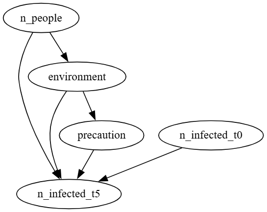
Figure: Pictorial representation of the Causal DAG in this example.
digraph CausalDAG {
  n_people -> n_infected_t5
  environment -> n_infected_t5
  n_people -> environment
  n_infected_t0 -> n_infected_t5
  environment -> precaution
  precaution -> n_infected_t5
}
3. Causal Test Cases
We then define a number of causal test cases to apply to the scenario-under-test. For example, supposing we expect mask wearing and hand washing to have a preventative effect:
mask_wearing_test = (X={precaution = None}, \Delta = {precaution = Mask}, Y = {-20% < n_infected_t5 < -10% })(Mask wearing is expected to result in between 10% and 20% fewer infections).hand_washing_test = (X={precaution = None}, \Delta = {precaution = Hand Washing}, Y = {-40% < n_infected_t5 < -25%})(Hand washing is expected to result in between 25% and 40% fewer infections).
To run these test cases experimentally, we need to execute both
Xand\Delta(X)- that is, with and without the interventions. Since the only difference between these test cases is the intervention, we can conclude that the observed difference inn_infected_t5was caused by the interventions. While this is the simplest approach, it can be extremely inefficient at scale, particularly when dealing with complex software such as computational models.To run these test cases observationally, we need valid observational data for the scenario-under-test. This means we can only use executions with between 20 and 30 people, a square environment of size betwen 20x20 and 40x40, and where a single person was initially infected. In addition, this data must contain executions both with and without the intervention. Next, we need to identify any sources of bias in this data and determine a procedure to counteract them. This is achieved automatically using graphical causal inference techniques that identify a set of variables that can be adjusted to obtain a causal estimate. Finally, for any categorical biasing variables, we need to make sure we have executions corresponding to each category otherwise we have a positivity violation (i.e. missing data). In the worst case, this at least guides the user to an area of the system-under-test that should be executed.
4. Causal Testing
After obtaining suitable test data, we can now apply causal inference. First, as described above, we use our causal graph to identify a set of adjustment variables that mitigate all bias in the data. Next, we use statistical models to adjust for these variables (implementing the statistical procedure necessary to isolate the causal effect) and obtain the desired causal estimate. Depending on the statistical model used, we can also generate 95% confidence intervals (or confidence intervals at any confidence level for that matter).
In our example, the causal DAG tells us it is necessary to adjust for
environmentin order to obtain the causal effect ofprecautiononn_infected_t5. Supposing the relationship is linear, we can employ a linear regression model of the formn_infected_t5 ~ p0*precaution + p1*environmentto carry out this adjustment. If we use experimental data, only a single environment is used by design and therefore the adjustment has no impact. However, if we use observational data, the environment may vary and therefore this adjustment will look at the causal effect within different environments and then provide a weighted average, which turns out to be the partial coefficientp0.
5. Test Oracle Procedure
After conducting causal inference, all that remains is to ascertain whether the causal effect is expected or not. In our example, this is simply a case of checking whether the causal effect on
n_infected_t5falls within the specified range. However, in the future, we may wish to implement more complex oracles.